Module 1: Introduction and Data Science Theory

Intro

Key Points

• Data science is about using data to make decisions that drive actions.
• Data science involves:

1. Finding data
2. Acquiring data
3. Cleaning and transforming data
4. Understanding relationships in data
5. Delivering value from data

• Predictive analytics is about using past data to predict future values.
• Prescriptive analytics is about using those predictions to drive decisions.

Data Science Process

Key Points

The data science process involves:

1. Data selection.
2. Preprocessing.
3. Transformation.
4. Data Mining.
5. Interpretation and evaluation.

It is an iterative process in which some, or all, steps may be repeated.

Intro to Machine Learning

Key Points

Classification and Regression

• Classification and regression use data with known values to train a machine learning model so that it can identify unknown values for other data entities with similar attributes.
• Classification is used to identify Boolean (True/False) values. Regression is used to identify real numeric values. So a question like "In this a chair?" is a classification problem, while "How much does this person earn?" is a regression problem.
• Both classification and regression are examples of supervised learning, in which a machine learning model is trained using a set of existing, known data values. The basic principle is as follows:

1. Define data entities based on a collection (or vector) of numeric variables (which we call features) and a single predictable value (which we call a label). In classification, the label has a value of -1 for False and +1 for True.
2. Assemble a training set of data that contains many entities with known feature and label values - we call the set of feature values x and the label value y.
3. Use the training set and a classification or regression algorithm to train a machine learning model to determine a function (which we call f) that operates on x to produce y.
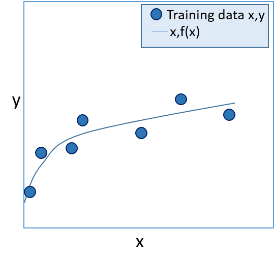
4. The trained model can now use the function f(x)=y to calculate the label (y) for new entities based on their feature values (x). In classification, if y is positive, the label is True; if y is negative, the label is False. The function can be visualized as a line on a chart, showing the predicted y value for a given x value. The predicted values should be close to the actual known values for the training set, as shown in figure 1 below.
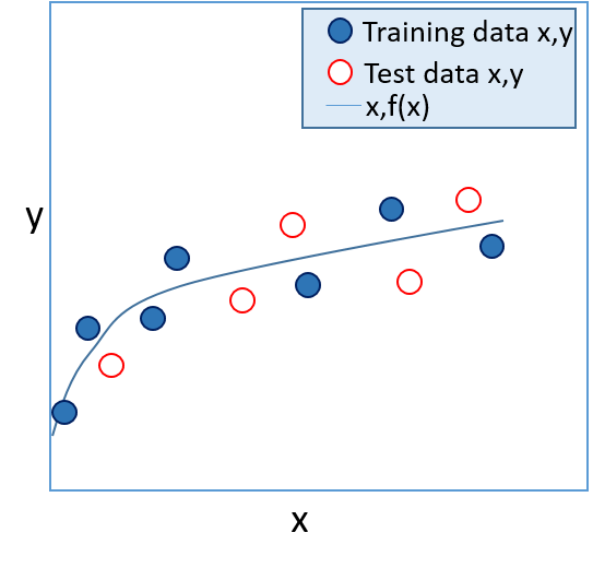
5. You can evaluate the model by applying it to a set of test data with known label (y) values. The accuracy of the model can be validated by comparing the value calculated by f(x) with the known value for y, as shown in figure 2.

Figure 1: A trained model	Figure 2: A validated model

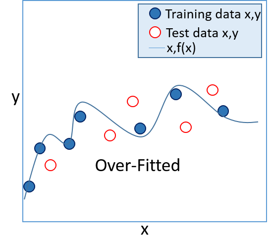
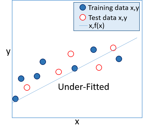
• In a supervised learning model, the goal is to produce a function that accurately calculates the known label values for the training set, but which is also generalized enough to predict accurately for known values in a test set (and for unknown values in production data). Functions that only work accurately with the training data are referred to as "over-fitted", and functions that are too general and don't match the training data closely enough are referred to as "under-fitted". In general, the best functions are ones that are complex enough to accurately reflect the overall trend of the training data, but which are simple enough to calculate accurate values for unknown labels.

Figure 3: An over-fitted model	Figure 4: An under-fitted model

Clustering

• Clustering is an unsupervised learning technique in which machine learning is used to group (or cluster) data entities based on similar features.
• It is difficult to evaluate clustering models, because there is no training set with known values that you can use to train the model and compare its results.

Recommendation

• Recommender systems are machine learning solutions that match individuals to items based on the preferences of other similar individuals, or other similar items that the individual is already known to like.
• Recommendation is one of the most commonly used forms of machine learning.

Regression

Key Points

• When operating on the data in the training and test datasets, the difference between the known y value and the value calculated by f(x) must be minimized. In other words, for a single entity, y - f(x) should be close to zero. This is controlled by the values of any baseline variables (b) used in the function.
• For various reasons, computers work better with smooth functions than with absolute values, so the values are squared. In other words, (y - f(x))² should be close to zero.
• To apply this rule to all rows in the training or test data, the squared values are summed over the whole dataset, so ∑(y_i - f(x_i))² should be close to zero. This quantity is known as the sum of squares errors (or SSE). The regression algorithm minimizes this by adjusting the values of baseline variables (b) used in the function.
• Minimizing the SSE for simple linear regression models (where there is only a single x value) generally works well, but when there are multiple x values, it can lead to over-fitting. To avoid this, the you can use ridge regression, in which the regression algorithm adds a regularization term to the SSE. This helps achieve a balance of accuracy and simplicity in the function.
• Support vector machine regression is an alternative to ridge regression that uses a similar technique to minimize the difference between the predicted f(x) values and the known y values.
• To determine the best algorithm for a specific set of data, you can use cross-validation, in which the data is divided into folds, with each fold in turn being used to test algorithms that are trained on the other folds.
• To determine the optimal value for a parameter (k) for an algorithm, you can use nested cross-validation, in which one of the folds in the training set is used to validate all possible k values. This process is repeated so that each fold in the training set is used as a validation fold. The best result is then tested with the test fold, and the whole process is repeated again until every fold has been used as the test fold.

Classification

Key Points

• For a classification function to work accurately, when operating on the data in the training and test datasets, the number of times that the sign of f(x) does not equal y must be minimized. In other words, for a single entity, if y is positive, f(x) should be positive; and if y is negative, f(x) should be negative. Formally, we need to minimize cases where y ≠ sign(f(x)).
• Because same-signed numbers when multiplied together always produce a positive, and numbers of different signs multiplied together always produce a negative, we can simplify our goal to minimize cases where yf(x) < 0; or for the whole data set ∑_iy_if(x_i) < 0. This general approach is known as a loss function.
• As with regression algorithms, some classification algorithms add a regularization term to avoid over-fitting so that the function achieves a balance of accuracy and simplicity.
• Each classification algorithm (for example AdaBoost, Support Vector Machines, and Logistic Regression) uses a specific loss function implementation, and it's this that distinguishes classification algorithms from one another.
• Decision Trees are classification algorithms that define a sequence of branches. At each branch intersection, the feature value (x) is compared to a specific function, and the result determines which branch the algorithm follows. All branches eventually lead to a predicted value (-1 or +1). Most decision trees algorithms have been around for a while, and many produce low accuracy. However, boosted decision trees (AdaBoost applied to a decision tree) can be very effective.
• You can use a "one vs. all" technique to extend binary classification (which predicts a Boolean value) so that it can be used in multi-class classification. This approach involves applying multiple binary classifications (for example, "is this a chair?", "is this a bird?", and so on) and reviewing the results produced by f(x) for each test. Since f(x) produces a numeric result, the predicted value is a measure of confidence in the prediction (so for example, a high positive result for "is this a chair?" combined with a low positive result for "is this a bird?" and a high negative result for "is this an elephant?" indicates a high degree of confidence that the object is more likely to be a chair than a bird, and very unlikely to be an elephant.)
• When the training data is imbalanced (so a high proportion of the data has the same True/False value for y) , the accuracy of the classification algorithm can be compromised. To overcome this problem, you can "over-sample" or "weight" data with the minority y value to balance the algorithm.
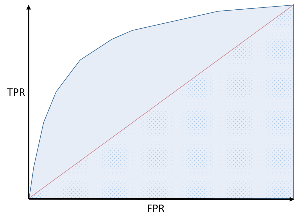
• The quality of a classification model can be assessed by plotting the True Positive Rate (predicted positives / actual positives) against the False Positive Rate (predicted negatives / actual negatives) for various parameter values on a chart to create a receiver operator characteristic (ROC) curve. The quality of the model is reflected in the area under the curve. The larger this area is than the area under a straight diagonal line (representing a 50% accuracy rate that can be achieved purely by guessing), the better the model; as shown below:

Clustering

Key Points

• Clustering groups data entities based on their feature values. Each data entity is described as a vector of one or more numeric features (x), which can be used to plot the entity as a specific point.
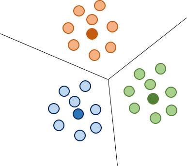
• K-Means clustering is a technique in which the algorithm groups the data entities into a specified number of clusters (k). To begin, the algorithm selects k random centroid points, and assigns each data entity to a cluster based on the shortest distance to a centroid. Each centroid is then moved to the central point (i.e. the mean) of its cluster, and the distances between the data entities and the new centroids are evaluated, with entities reassigned to another cluster if it is closer. This process continues until every data entity is closer to the mean centroid of its cluster than to the centroid of any other cluster. The following image shows the result of K=Means clustering with a k value of 3:

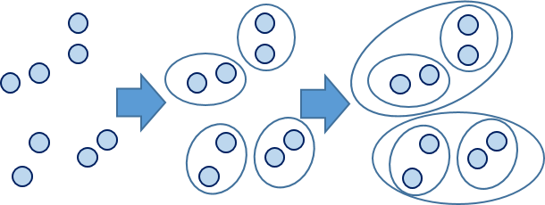
• Hierarchical Agglomerative Clustering is an alternative clustering technique in which the point representing each data entity begins as its own cluster. Each cluster is then merged with the cluster closest to it, and this merging process continues iteratively. The following image illustrates the process of Hierarchical Agglomerative Clustering.

• The distance metric used to determine how "close" points are to one another is an important aspect of clustering. The simplest way to conceptualize the entities is as points in Euclidean space (multidimensional coordinates), and measure the simple distance between the points; but other distance metrics can also be used.

Recommendation

Key Points

• Recommender systems are often based on a matrix of ratings that users give to items, as shown in the following image:

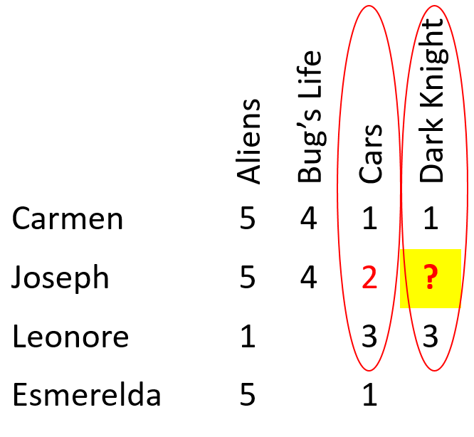
• User-based collaborative filtering predicts unknown ratings based on ratings of other users who gave similar ratings for other items. For example, in the following image, the Joseph's rating for The Dark Knight can be predicted based on the ratings given for that movie by other users who gave similar ratings to Joseph for other movies. In this case, Carmen gave similar ratings for Aliens and A Bug's Life to the ratings that Joseph gave for those movies, so it's reasonable to predict that Joseph will give The Dark Knight a similar rating to Carmen's.

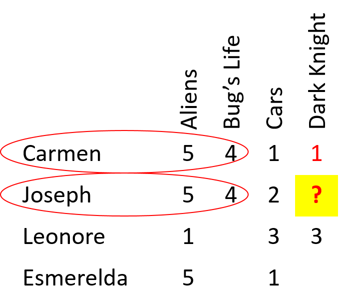
• Item-based collaborative filtering predicts unknown ratings based on ratings for other items that received similar ratings from other users. For example, in the following image, Cars and The Dark Knight have received similar ratings from each user that has rated both. It is therefore reasonable to predict that Joseph will give The Dark Knight a similar rating to the one he gave to Cars.

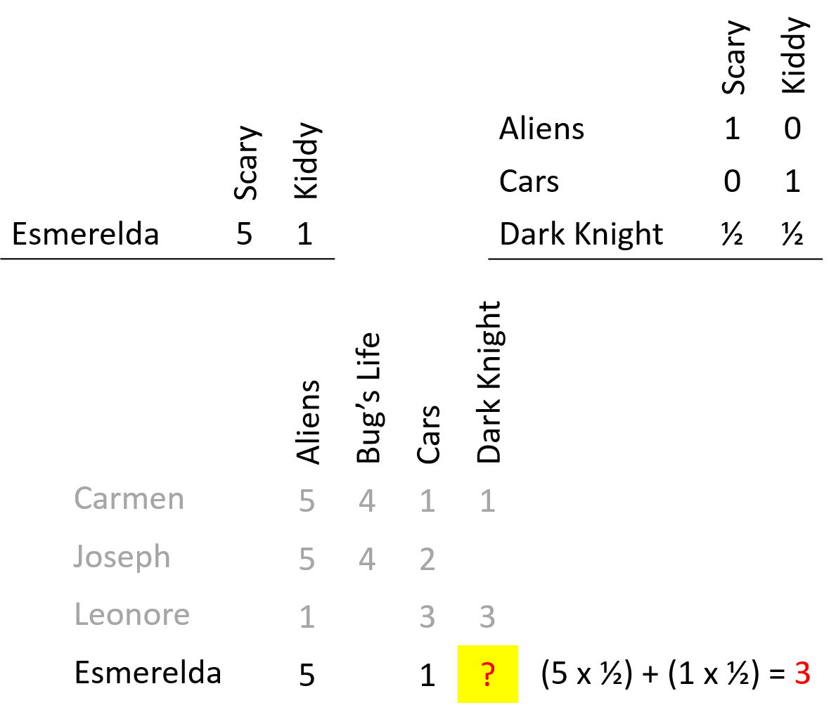
• Matrix Factorization attempts to determine latent features for items and users, and correlate them to predict ratings. For example, features for "scariness" and "kiddiness" could be determined for movies (so Aliens is a scary movie, Cars is a kid's movie, and The Dark Knight has an even degree of "scariness" and "kiddiness"). Based on her known ratings, Esmerelda has a high "scariness" feature (she likes scary movies) and a low "kiddiness" feature (she dislikes kid's movies). By applying these derived latent features, a predicted rating that Esmerelda would give to The Dark Knight can be calculated by multiplying the "scariness" and "kiddiness" features for her and the movie, and adding the results together.